Third Harmonic Generation in bulk Silicon
In this tutorial we will calculate third harmonic generation (THG) in bulk Silicon. Calculation of third harmonic generation proceeds in similar way to the SHG calculations. DFT input can be found here (abinit or quantum espresso).
We import the wave-functions as explained in the SHG tutorial, then perform the setup using only 1000 plane waves.
We are interested in the \( \chi^{(3)}_{1111} \) therefore we consider an external field in direction [1, 0, 0] (equivalent to [x,0,0]).
We remove all the symmetries not compatible with the external field plus the time-reversal symmetry by doing ypp -n:
Then you go in the FixSymm folder, run again the setup (as explained in the first tutorial) and then generate the input file with the command lumen -u -V qp -F input.in:
We calculate the \( \chi^{(3)}_{1111} \) only on 6 frequencies, but calculations can be extened to larger frequency range. We introduce a scissor operator of 0.6 eV in such a way to reproduce the gap of bulk silicon. Notice that we increased the field intensity in such a way to improve the ratio between non-linear response and numerical noise.
Now that you have created the file input.in you can run the non-linear optics calculation with the command:
when the simulation will end, it will have produced the files SAVE/ndb.Nonlinear.
Results can be analized in the same way of the SHG, using the command ypp -u:
This time we increase the dephasing time to 40 fs in such a way to have a clean third-harminic response.
Hereafter we report the result with the 8x8x8 k-points sampling and the converged result with the 24x24x24 k-points sampling: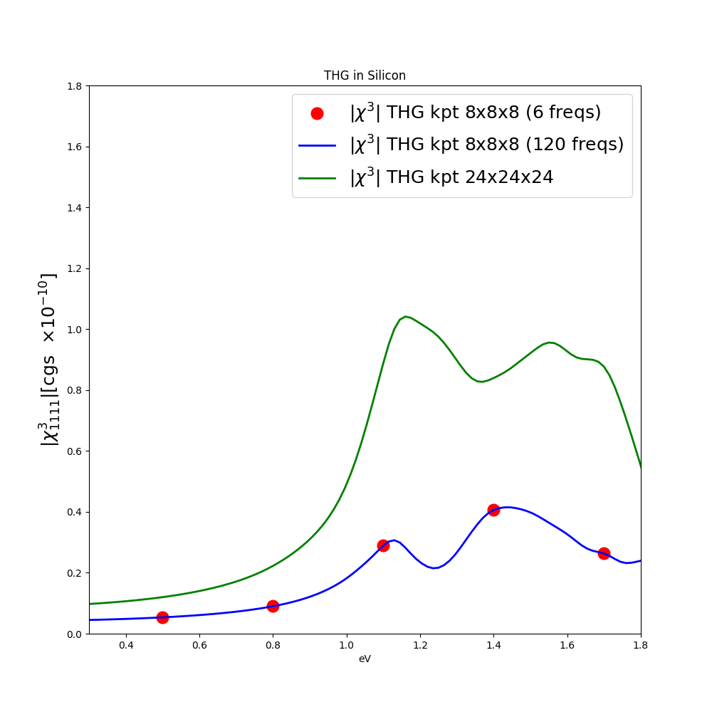
We are interested in the \( \chi^{(3)}_{1111} \) therefore we consider an external field in direction [1, 0, 0] (equivalent to [x,0,0]).
We remove all the symmetries not compatible with the external field plus the time-reversal symmetry by doing ypp -n:
fixsyms                      # [R] Reduce Symmetries
% Efield1
 1.00     | 0.00     | 0.00     |        # First external Electric Field
%
% Efield2
 0.00     | 0.00     | 0.00     |        # Additional external Electric Field
%
#RmAllSymm                   # Remove all symmetries
RmTimeRev                    # Remove Time Reversal
Then you go in the FixSymm folder, run again the setup (as explained in the first tutorial) and then generate the input file with the command lumen -u -V qp -F input.in:
nlinear                      # [R NL] Non-linear optics
% NLBands
  1 | 7 |                   # [NL] Bands
%
NLstep=   0.0100       fs    # [NL] Real Time step length
NLtime=-1.000000       fs    # [NL] Simulation Time
NLintegrator= "CRANKNIC"     # [NL] Integrator ("EULEREXP/RK4/RK2EXP/HEUN/INVINT/CRANKNIC")
NLCorrelation= "IPA"         # [NL] Correlation ("IPA/HARTREE/TDDFT/LRC/JGM/HF/SEX")
NLLrcAlpha= 0.000000         # [NL] Long Range Correction
% NLEnRange
 0.200000 | 2.000000 |  eV    # [NL] Energy range
%
NLEnSteps=  6               # [NL] Energy steps
NLDamping= 0.200000    eV    # [NL] Damping
NLGvecs=  941          RL    # [NL] Number of G vectors in NL dynamics for Hartree/TDDFT
NLInSteps= 1                 # [NL] Intensity steps for Richardson extrap. (1-3)
% ExtF_Dir
 1.000000 | 0.000000 | 0.000000 |        # [NL ExtF] Versor
%
ExtF_Int=0.1000E+8         kWLm2 # [NL ExtF] Intensity
ExtF_kind= "SOFTSIN"         # [NL ExtF] Kind(SIN|SOFTSIN|RES|ANTIRES|GAUSS|DELTA|PULSE)
% GfnQP_E
 0.600000 | 1.000000 | 1.000000 |        # [EXTQP G] E parameters  (c/v) eV|adim|adim
%
We calculate the \( \chi^{(3)}_{1111} \) only on 6 frequencies, but calculations can be extened to larger frequency range. We introduce a scissor operator of 0.6 eV in such a way to reproduce the gap of bulk silicon. Notice that we increased the field intensity in such a way to improve the ratio between non-linear response and numerical noise.
Now that you have created the file input.in you can run the non-linear optics calculation with the command:
lumen -F input.in
when the simulation will end, it will have produced the files SAVE/ndb.Nonlinear.
Results can be analized in the same way of the SHG, using the command ypp -u:
nonlinear                    # [R] NonLinear Optics Post-Processing
Xorder=  5                   # Max order of the response functions
% TimeRange
 40 | -1.00000 | fs    # Time-window where processing is done
%
ETStpsRt= 200                # Total Energy steps
% EnRngeRt
 0.00000 | 10.00000 | eV    # Energy range
%
DampMode= "NONE"             # Damping type ( NONE | LORENTZIAN | GAUSSIAN )
DampFactor=  0.10000   eV    # Damping parameter
This time we increase the dephasing time to 40 fs in such a way to have a clean third-harminic response.
Hereafter we report the result with the 8x8x8 k-points sampling and the converged result with the 24x24x24 k-points sampling: