Second Harmonic Generation in AlAs
In this tutorial we will calculate the second harmonic generation of bulk AlAs. The first six step of this tutorials are the same of the one on linear-response with the only different that we will work on AlAs and we will use Abinit to generate the Kohn-Sham wave-functions. The DFT input are available here: ABINIT or QuantumEspresso.
You can run the DFT calculation with ABINIT with the command:
1) Real-time simulation for the SHG
You can generate the input file with the command yambo_nl -u:
The line |1.000000 | 1.000000 | 0.000000 | # [NL ExtF] Versor referees to the direction of the external field (x,y,0). At present only an external field is present but the code can be easily generalized to deal with more fields.
The default parameters of Yambo/Lumen are already tuned for second-harmonic generation, so the only thing you have to change is the bands range, between 3 and 6 and the energy range between 1.0-5.0 eV and the number of energy steps in this interval that we set to 10. Notice that you cannot set to zero the lowest value of the energy range because this will requires a simulation that lasts infinite time, see below. Finally consider that Yambo/Lumen performs a separate calculation for each frequency, so if you set many energy steps the computational time grows linearly with this number.
Run yambo_nl. Calculations will take about fifteen on a single processor PC, you have time to study the next section that explains how non-linear response is extracted from the real-time simulations.
2) Non-linear response with Yambo/Lumen
In order to calculate the non-linear response the system is excited with different laser fields with a sinusoidal shape at frequencies \( \omega_1, \omega_2, .... , \omega_n \) determined by the parameters NLEnRange and NLEnSteps. A dephasing term is added to the Hamiltonian \(\gamma=NLDamping\) to simulate a finite broadening and to remove the eigenmodes that are excited by the sudden turning on of the external field. After the dephasing time the outgoing signal is analyzed to extract the non-linear coefficients as shown in the figure below: 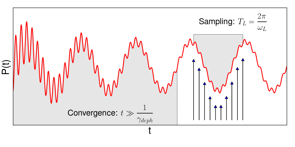
In the report file r_nlinear you will find the length of the dephasing part and of the sampling one:
3) Analysis of the results
In the sampling region we suppose that the polarization can be written as: $$\bf{P}(t) = \sum_{n=-\infty}^{+\infty} \bf{p}_n e^{-i\omega_n t} $$ where the coefficient \(\bf{p}_1,...,\bf{p}_n\) are related to \(\chi^{(1)},...,\chi^{(n)}\). We sample the polarization signal at different times and invert the previous equation by truncating the sum at a finite order.
This is done with the command ypp_nl -u that automatically produce an input with the correct values:
where Xorder is the order where the previous sum is truncated, and the TimeRange specifies the sampling region. Notice that differently from the first tutorial in this case we do not need Damping in ypp because we already included it in the real-time dynamics. Run ypp and it will produce a file called o.YPP-X_probe_order_2 with the \( \chi^2_{xyz}\), columns 6 and 7. You can plot the result:
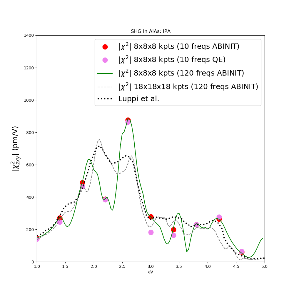
and compare it with the \( \chi^2_{zxy}\) calculated with more frequencies and with the converged result on a 18x18x18 k-point grid and bands between 2 and 10.
In the figure you can find also the comparison with the results of Luppi et al. PRB B, 82, 235201(2010).
Notice that the QuantumEspresso results are slightly different from the Abinit ones. This is due to the different pseudo-potential employed in the calculations, if pseudopotentials were the same calculation would have been identical.
You can download the script to generate this plot and the converged results here.
You can run the DFT calculation with ABINIT with the command:
abinit < AlAs.in > output_AlAsor using QuantumEspresso:
pw.x -inp AlAs.scf.in > output_scf
pw.x -inp AlAs.nscf.in > output_scf
and then import the ABINIT wave-function with the command:
a2y -F alas-o_DS2_KSSand the QuantumEspresso one, in the folder AlAs.save with the command:
p2y -F data-file-schema.xmlNow you proceed in the same wave of the previous tutorial (from point 2 to 6) considering an external field in the [1,1,0] direction.
1) Real-time simulation for the SHG
You can generate the input file with the command yambo_nl -u:
nlinear                      # [R NL] Non-linear optics
% NLBands
  3 | 6 |                   # [NL] Bands
%
NLstep=   0.0100       fs    # [NL] Real Time step length
NLintegrator= "INVINT"       # [NL] Integrator ("EULEREXP/RK4/RK2EXP/HEUN/INVINT/CRANKNIC")
NLCorrelation= "IPA"         # [NL] Correlation ("IPA/HARTREE/TDDFT/LRC/JGM/SEX/HF")
NLLrcAlpha= 0.000000         # [NL] Long Range Correction
% NLEnRange
  1.000000 | 5.000000 | eV    # [NL] Energy range
%
NLEnSteps= 10                # [NL] Energy steps
NLDamping= 0.150000    eV    # [NL] Damping
% ExtF_Dir
 1.000000 | 1.000000 | 0.000000 |        # [NL ExtF] Versor
ExtF_kind= "SOFTSIN"         # [NL ExtF] Kind(SIN|SOFTSIN|RES|ANTIRES|GAUSS|DELTA|QSSIN)
The line |1.000000 | 1.000000 | 0.000000 | # [NL ExtF] Versor referees to the direction of the external field (x,y,0). At present only an external field is present but the code can be easily generalized to deal with more fields.
The default parameters of Yambo/Lumen are already tuned for second-harmonic generation, so the only thing you have to change is the bands range, between 3 and 6 and the energy range between 1.0-5.0 eV and the number of energy steps in this interval that we set to 10. Notice that you cannot set to zero the lowest value of the energy range because this will requires a simulation that lasts infinite time, see below. Finally consider that Yambo/Lumen performs a separate calculation for each frequency, so if you set many energy steps the computational time grows linearly with this number.
Run yambo_nl. Calculations will take about fifteen on a single processor PC, you have time to study the next section that explains how non-linear response is extracted from the real-time simulations.
2) Non-linear response with Yambo/Lumen
In order to calculate the non-linear response the system is excited with different laser fields with a sinusoidal shape at frequencies \( \omega_1, \omega_2, .... , \omega_n \) determined by the parameters NLEnRange and NLEnSteps. A dephasing term is added to the Hamiltonian \(\gamma=NLDamping\) to simulate a finite broadening and to remove the eigenmodes that are excited by the sudden turning on of the external field. After the dephasing time the outgoing signal is analyzed to extract the non-linear coefficients as shown in the figure below:
  Dephasing Time          [fs]: 43.880793
  Sampling  Time          [fs]:  4.185667
  Total simulation time   [fs]: 48.066460
The length of the dephasing interval is inversely proportional to the damping term $$T_{depth} \simeq 1/\gamma$$ while the length of the sampling is dictated by the smallest frequency we are interested in: $$T_{samp} \simeq 1/\omega_1$$. For this reason if \( \omega_1=0 \) or \(\gamma = 0\) simulation time goes to infinity. You can have a look to the file src/nloptics/NL_initialize.F to see how simulation lengths are defined.
3) Analysis of the results
In the sampling region we suppose that the polarization can be written as: $$\bf{P}(t) = \sum_{n=-\infty}^{+\infty} \bf{p}_n e^{-i\omega_n t} $$ where the coefficient \(\bf{p}_1,...,\bf{p}_n\) are related to \(\chi^{(1)},...,\chi^{(n)}\). We sample the polarization signal at different times and invert the previous equation by truncating the sum at a finite order.
This is done with the command ypp_nl -u that automatically produce an input with the correct values:
nonlinear                    # [R] NonLinear Optics Post-Processing
Xorder=  4                   # Max order of the response functions
% TimeRange
 43.89079 | -1.00000 | fs    # Time-window where processing is done
%
ETStpsRt= 200                # Total Energy steps
% EnRngeRt
  0.00000 | 10.00000 | eV    # Energy range
%
DampMode= "NONE"             # Damping type ( NONE | LORENTZIAN | GAUSSIAN )
DampFactor=  0.10000   eV    # Damping parameter
where Xorder is the order where the previous sum is truncated, and the TimeRange specifies the sampling region. Notice that differently from the first tutorial in this case we do not need Damping in ypp because we already included it in the real-time dynamics. Run ypp and it will produce a file called o.YPP-X_probe_order_2 with the \( \chi^2_{xyz}\), columns 6 and 7. You can plot the result: