Theory

The Lumen code implements a real-time effective Schrödinger equation, where the coupling between electrons and external field is described by means of modern theory of polarization[1]:

$$ i \hbar \frac{\partial}{\partial t} | v_{i \mathbf{k}} \rangle = \left( \hat H^{sys}_{\mathbf k} + i e \mathcal{E}(t) \cdot \partial_{\mathbf k} \right ) | v_{i \mathbf{k}} \rangle $$

Where \( | v_{i \mathbf{k}} \rangle \) are the time-dependent valence bands, \( H^{sys}_{\mathbf k} \) is the Hamiltonian, \( \mathcal{E}(t)\) is the external field and the term \( i e \partial_{\mathbf k} \) corresponds to the dipole operator in periodic systems. For more details on this last term see references [2-3].
Differently from other codes the equation of motion of Lumen are in the length gauge and not in the velocity one. If you want to know more about advantages and disadvantages of the two gauges read section 2.7 of ref. [8].
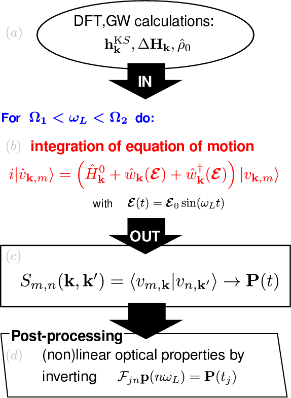
The Hamiltonian and the initial wave-functions are obtained from DFT. Then in order to obtain linear and non-linear response the system is excited with a sinusoidal laser field and the time dependent polarization is calculated. Hereafter a schematic representation of the calculations:

In the previous equation the model Hamiltonian chosen for \( H^{\text{sys}}_{\mathbf k} \) determines the level of approximation in the description of correlation effects in the linear and nonlinear spectra.

Hamiltonians

Lumen code can use different models for the system Hamiltonian:

1. The independent-particle (IP) model, $$ H^{\text{IP}}_{\mathbf k} \equiv H^{\text{KS}}_{\mathbf k} $$ where \( H^{\text{KS}}_{\mathbf k} \) is the unperturbed KS Hamiltonian and we consider the KS system as a system of independent particles.
2. The QP model, $$ H^{\text{QP}}_{\mathbf k} \equiv H^{\text{KS}}_{\mathbf k} + \Delta H_{\mathbf k}. $$ where GW corrections or scissor operator, estimated from the Many-Body Perturbation Theory (ref. [4]), has been applied to the KS eigenvalues.
3. The RPA model, $$ H^{\text{RPA}}_{\mathbf k} \equiv H^{\text{KS}}_{\mathbf k} + V_h(\mathbf r)[\Delta\rho], $$ The term \( V_h(\mathbf r)[\Delta\rho] \) is the time-dependent Hartree potential and is responsible for the local-field effects originating from system inhomogeneities, and \( \Delta \rho \equiv \rho(\mathbf r;t)-\rho(\mathbf r;t=0) \) is the variation of the electronic density.
4. The Time Dependent-Density Functional Theory (TD-DFT) model, at present only for LDA or GGA functionals: $$ H^{\text{RPA}}_{\mathbf k} \equiv H^{\text{KS}}_{\mathbf k} + V_h(\mathbf r)[\Delta\rho] + V_{xc}(\mathbf r)[\Delta\rho] $$ The term \( V_{xc}(\mathbf r)[\Delta\rho] \) is the time-dependent exchange-correlation potential.
5. The Time Dependent-Density Polarization Function Theory (TD-DPFT) model, at present different functionals are implemented in Lumen, for more details see ref. [5]: $$ H^{\text{RPA}}_{\mathbf k} \equiv H^{\text{KS}}_{\mathbf k} + V_h(\mathbf r)[\Delta\rho] + V_{xc}(\mathbf r)[\Delta\rho] -\Omega \mathcal{E}^s(t) \cdot \nabla_{\mathbf k} $$

where \( \mathcal{E}^s(t) \) is the Kohn-Sham macroscopic field (see ref.[5-6]).

Non-linear susceptibilities

During the time evolution the bulk polarization is calculated by means of King-Smith Vanderbilt formula (ref. [7]) and the nonlinear susceptibilities are obtained by inversion of the Fourier matrix as described in ref. [3]: $$ P=P^0 + \chi^{(1)} E + \chi^{(2)} E^2 + \chi^{(3)} E^3 + O(E^4)$$ Notice that the finite broadening in the spectra is obtained by adding a dephasing operator in the original Hamiltonian (ref. [3]).

References:

- Manifestations of Berry’s phase in molecules and condensed matter, Raffaele Resta, J. Phys.: Condens. Matter, 12,R107–R143(2000)
- Dynamics of Berry-phase polarization in time-dependent electric fields, I. Souza, J. Iniguez, and D. Vanderbilt, Phys. Rev. B 69, 085106 (2004)
- Nonlinear optics from an ab initio approach by means of the dynamical Berry phase: Application to second- and third-harmonic generation in semiconductors, C. Attaccalite, M. Grüning, Phys. Rev. B, 88, 235113 (2013)
- The GW method, F. Aryasetiawan, O. Gunnarsson, Rep. Prog. Phys. 61, 237 (1998)
- Dielectrics in a time-dependent electric field: a real-time approach based on density-polarization functional theory, M. Grüning, D. Sangalli, C. Attaccalite, Phys. Rev. B 94, 035149 (2016)
- Functional theory of extended Coulomb systems, R. M. Martin and G. Ortiz, Phys. Rev. B 56, 1124 (1997)
- Theory of polarization of crystalline solids, R.D. King-Smith, D. Vanderbilt, Phys. Rev. B 47, 1651(R) (1993)
- Non-linear response in extended systems: a real-time approach, C. Attaccalite (2017)