Next: Bibliography
Up: thesis
Previous: Determinant derivatives
Contents
Error Analysis due to finite time step in the GLE integration in a simple case
When we discretize the equation 5.13 we introduce an error due to the finite integration time step  . Following the idea of Ref. (111) we can evaluate this error analytically in the case of a simple harmonic oscillator.
Consider the equation:
. Following the idea of Ref. (111) we can evaluate this error analytically in the case of a simple harmonic oscillator.
Consider the equation:
 |
(E.1) |
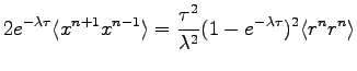
We are interested in a statistically stationary process and so we proceed to evaluate mean average energies and correlation functions as function of
. To do so we multiply the equation E.1 for  and
and  , respectively, and then take the average. We obtain the following pair of equations:
Becuase we are interested in the equilibrium distribution, we can assume that
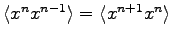 and
and
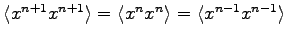 .
Thus we have three unknown quantities
.
Thus we have three unknown quantities
 ,
,
 and
and
 .
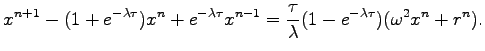
To get a third relation among this quantities we square the Eq. E.1 to obtain the relation:
.
To get a third relation among this quantities we square the Eq. E.1 to obtain the relation:
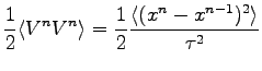
After solving this equation system we can evaluate the potential and the kinetic energy:
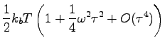
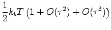
It is easy to show that in the limit of small
the potential and the kinetic energies converge to:
This show that at least in this simple model the impulse integrator leads to a quadratic error in
in both kinetic and poterntial energy.
Next: Bibliography
Up: thesis
Previous: Determinant derivatives
Contents
Claudio Attaccalite
2005-11-07
![$\displaystyle \langle x^{n+1} x^{n} \rangle + \left [ \frac{\tau \omega^2 }{\la...
... ] \langle x^{n} x^{n} \rangle +e^{-\lambda \tau} \langle x^{n-1} x^{n} \rangle$](img778.png)
![$\displaystyle \langle x^{n+1} x^{n-1} \rangle -(1+e^{-\lambda \tau }) \langle x...
...\lambda \tau} - 1) +
e^{-\lambda \tau} \right ] \langle x^{n-1} x^{n-1} \rangle$](img779.png)
![$\displaystyle \left [ \frac{\tau \omega^2 }{\lambda} (e^{-\lambda \tau} -1 ) - ...
...tau}) \right ] \left(1+ e^{-\lambda \tau} \right) \langle x^{n+1} x^{n} \rangle$](img786.png)
![$\displaystyle \left [ 1 + e^{-2\lambda \tau } + \left ( \frac{\tau \omega^2 }{\...
...da \tau} )+(1+e^{-\lambda \tau}) \right )^2 \right] \langle x^{n} x^{n} \rangle$](img787.png)

![$\displaystyle \frac{1}{\tau^2} \left [ \langle x^{n} x^{n} \rangle - \langle x^{n} x^{n-1} \rangle \right]$](img793.png)