


Next: Practical implementation of the
Up: Canonical ensemble by Generalized
Previous: Canonical ensemble by Generalized
Contents
In the literature there are different algorithms to integrate numerically the Generalized Langevin Equation. The most common ones are the BBK (91), vGB82 (92) and the Impulse Integrator (LI) (93). All of them, in the limit of Newtonian dynamics, as
 , reduce to the well known Verlet method:
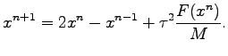 |
(5.18) |
Although these methods offer good numerical accuracy, other criteria have to be considered for the choice of the algorithm. In our approach the friction is related to the quantum Monte Carlo noise, and so, in order to simulate low temperate phases, it can happen that we are forced to use a large friction matrix. Due to this, an integration algorithm that allows to work accurately with a large friction is required. In the limit of large friction, or equivalently
 the eq. 5.4 reduces to the simple Brownian dynamics. In this case the BBK scheme becomes unconditionally unstable (94), and this fact automatically excludes this algorithm. Instead the other two schemes reduce respectively to the second-order explicit Adams formula and to the Euler-Maruyama method (see Ref. (93)).
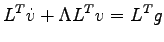
In this thesis we have decided to use the Impulse Integrator proposed by Skell and Izaguirre (93) that achieves a good accuracy (see Appendix E) and it is simple to implement. Moreover in order to integrate the Langevin dynamics 5.4 we have generalized this algorithm to a non-diagonal friction tensor. So we rewrite the equation 5.4 in the simpler form:
the eq. 5.4 reduces to the simple Brownian dynamics. In this case the BBK scheme becomes unconditionally unstable (94), and this fact automatically excludes this algorithm. Instead the other two schemes reduce respectively to the second-order explicit Adams formula and to the Euler-Maruyama method (see Ref. (93)).
In this thesis we have decided to use the Impulse Integrator proposed by Skell and Izaguirre (93) that achieves a good accuracy (see Appendix E) and it is simple to implement. Moreover in order to integrate the Langevin dynamics 5.4 we have generalized this algorithm to a non-diagonal friction tensor. So we rewrite the equation 5.4 in the simpler form:
 |
(5.19) |
where  is the friction tensor and
 . The forces
  are evaluated with QMC,
  contains therefore the noise of the QMC evaluation of
  and a possible additional external generated noise.
The friction tensor is assumed to be determined without noise but can explicitly depend on the atomic positions.
5.1.
Then we factorize the matrix
and a possible additional external generated noise.
The friction tensor is assumed to be determined without noise but can explicitly depend on the atomic positions.
5.1.
Then we factorize the matrix
 , where
  is a diagonal matrix and
  contains the corresponding eigenvectors. Substituting this factorization into eq. 5.19:
 |
(5.20) |
Defining the vectors  we obtain:
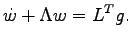 |
(5.21) |
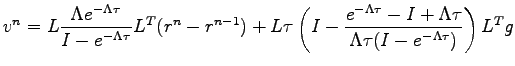
Now the equation is in the usual diagonal form with the new forces  . We assume that the friction matrix is slowly varying compared to the forces
  and so the usual integral scheme LI(93) is used for the variable
  . Finally the transformation
  is applied to come back to the original variables. The final integration formula is:
 |
(5.22) |
Then we can write the final formula to obtain velocities:
 |
(5.23) |
Next: Practical implementation of the
Up: Canonical ensemble by Generalized
Previous: Canonical ensemble by Generalized
Contents
Claudio Attaccalite
2005-11-07