Next: Setting the SR parameters
Up: Optimization Methods
Previous: Optimization Methods
Contents
Stochastic Reconfiguration (SR) technique was initial developed to partially solve the sign problem in lattice green function Monte Carlo (51) and then it was used as an optimization method for a generic trial-function (49,15). An important advantage of this technique is that we use more information about the trial-function than the simple steepest descent allowing a faster optimization of the many-body wave-function.
Given a generic trial-function  , not orthogonal to the ground state it is possible to obtain a new one closer to the ground-state by applying the operator
 to this wave-function for a sufficient large
  .
The idea of the Stochastic Reconfiguration is to change the parameters of the original trial-function in order to be as close as possible to the projected one.
.
The idea of the Stochastic Reconfiguration is to change the parameters of the original trial-function in order to be as close as possible to the projected one.
For this purpose we define:
where  is the projected one and
  is the new trail-function obtained changing variational parameters. We can write the equation eq. 2.2 as:
 |
(2.3) |
where
 and and  |
(2.4) |
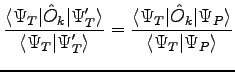
Now we want to choose the new parameters in such a way that
is as close as possible to
. Thus we require that a set of mixed average correlation function, corresponding to the two wave-functions 2.2, 2.1, are equal. Here we impose precisely that:
 |
(2.5) |
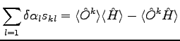
for  . This is equivalent to the equation system:
Because the equation for  is related to the normalization of the trial-function and this parameter doesn't effect any physical observable of the system, we can substitute
 from the first equation in the others:
 |
(2.8) |
where
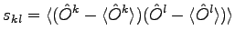 |
(2.9) |
The solution of this equation system defines a direction in the parameters space. If we vary parameters along this direction for a sufficient small step  we will decrease the energy.
The matrix  is calculated at each iteration through a standard variational
Monte Carlo sampling; the single iteration constitutes a small simulation
that will be referred in the following as ``bin''.
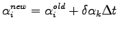
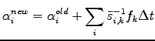
After each bin the wave function parameters
are iteratively updated according to
is calculated at each iteration through a standard variational
Monte Carlo sampling; the single iteration constitutes a small simulation
that will be referred in the following as ``bin''.
After each bin the wave function parameters
are iteratively updated according to
 |
(2.10) |
SR is similar to a standard steepest descent (SD) calculation, where
the expectation value of the energy
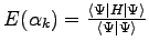 is optimized by iteratively changing
the parameters
is optimized by iteratively changing
the parameters  according to
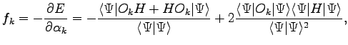
the corresponding derivatives of the energy (generalized forces):
according to
the corresponding derivatives of the energy (generalized forces):
 |
(2.11) |
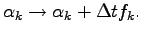
namely:
 |
(2.12) |
where
is a suitable small time step, which can be taken
fixed or determined at each iteration
by minimizing the energy expectation value.
Indeed the variation of the total energy  at each step is easily shown to
be negative for small enough
because, in this
limit
at each step is easily shown to
be negative for small enough
because, in this
limit
Thus the method certainly converges at the minimum when all the forces
vanish. In the SR we have
 |
(2.13) |
Using the analogy with the steepest descent, it is possible to show that
convergence to the energy minimum is reached when
the value of
is sufficiently small and
is kept constant for each iteration.
Indeed the energy variation for a small change of the parameters is:
and it is easily verified that the above term
is always negative because the reduced matrix  , as well
as
, as well
as  , is positive definite, being
an overlap matrix with all positive eigenvalues.
, is positive definite, being
an overlap matrix with all positive eigenvalues.
For a stable iterative method, such as the SR or the SD one,
a basic ingredient is that at each iteration the new parameters
 are close to the previous
  according to
a prescribed distance.
The fundamental difference between the SR minimization and the standard
steepest descent is just related to the
definition of this distance.
For the SD it is the usual one, that is defined by the Cartesian metric
according to
a prescribed distance.
The fundamental difference between the SR minimization and the standard
steepest descent is just related to the
definition of this distance.
For the SD it is the usual one, that is defined by the Cartesian metric
 , instead the SR
works correctly in the physical Hilbert space metric of the
wave function
, instead the SR
works correctly in the physical Hilbert space metric of the
wave function  , yielding
 namely the square distance between
the two wave functions corresponding to the two
different sets of variational
parameters
namely the square distance between
the two wave functions corresponding to the two
different sets of variational
parameters
 and
and
 .
Therefore, from the knowledge of the
generalized forces
.
Therefore, from the knowledge of the
generalized forces  , the most convenient change
of the variational parameters minimizes the functional
, the most convenient change
of the variational parameters minimizes the functional
 ,
where
is the linear change in the energy
,
where
is the linear change in the energy
 and
and
 is a Lagrange multiplier that allows a stable minimization
with small change
is a Lagrange multiplier that allows a stable minimization
with small change
 of the wave function
.
Then the final iteration (2.13) is
easily obtained.
of the wave function
.
Then the final iteration (2.13) is
easily obtained.
The advantage of SR compared with SD is obvious because sometimes a small
change of the variational parameters corresponds to a large change
of the wave function, and the SR takes into account this effect through
the Eq. 2.13.
In particular the method is useful when a non orthogonal basis set
is used, as we have in this thesis.
Moreover by using the reduced matrix
it is also possible to remove from
the calculation those parameters that imply some redundancy in
the variational space, as it is shown in the following sections of this chapter.
Subsections
Next: Setting the SR parameters
Up: Optimization Methods
Previous: Optimization Methods
Contents
Claudio Attaccalite
2005-11-07