


Next: Functional form of the
Up: Variational Monte Carlo
Previous: Variational Monte Carlo
Contents
In VMC the expectation value of operators different from the Hamiltonian is usually much less favorable and accurate than the one obtained for the energy. This is due to two kinds of errors: first the statistical one due to the finite sampling in the Monte Carlo integration that behaves as
 , where
  is the number of sampling points and second the systematic error ("bias") resulting from an approximated wave-function.
In order to understand the behavior of this errors we define the trial wave-function error,
 , where
  is the exact wave function.
In the case of the energy, applying the variational principle (see for instance ref. (28)), one finds that the systematic error
is the exact wave function.
In the case of the energy, applying the variational principle (see for instance ref. (28)), one finds that the systematic error  goes as
 , where
can be represented as:
, where
can be represented as:
 |
(1.4) |
Instead the statistical error is related to the variance of the operator on the trial wave-function  . For instance for the energy:
 |
(1.5) |
Using the equality:
 |
(1.6) |
it is easy to see that
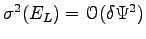 . Thus in the case of the energy both these errors vanish as
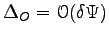
 . For any other operator that not commutes with the Hamiltonian,
is not anymore an eigenstate of
. For any other operator that not commutes with the Hamiltonian,
is not anymore an eigenstate of  and so the systematic error is
 while the statistical one is
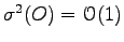 (see Ref. (30,29).
The situation is even worst if we consider atomic or molecular forces. In fact, let us derive the potential energy in the respect to an atomic position:
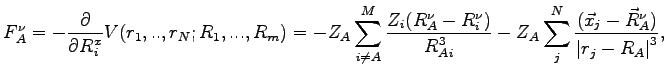 |
(1.7) |
the second term in the right-hand side of this equation is responsible for a infinite variance contribution.
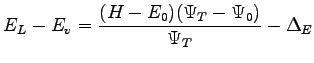
In order to overcome this problem Assaraf and Caffarel (31) proposed an original and ingenious solution. Denoting
an arbitrary hermitian operator they showed that is possible to define a new "renormalized" operator  such that:
The new operator
is obtained from the old one by adding to  another operator with zero expectation value and finite variance, namely:
![$\displaystyle \tilde O = O + \left [ \frac{\tilde H \tilde \Psi }{\tilde \Psi } - \frac{\tilde H \Psi_T}{ \Psi_T}\right ] \frac{\tilde{\Psi}}{\Psi_T},$](img89.png) |
(1.10) |
where  is an arbitrary Hermitian operator, and
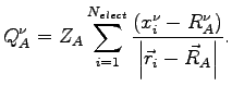
 is an auxiliary square-integrable function. In the case of atomic forces, the simplest and effective choice for
and
is:
is an auxiliary square-integrable function. In the case of atomic forces, the simplest and effective choice for
and
is:
with
 |
(1.13) |
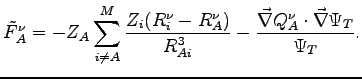
This particular form cancels the pathological part in the bare force 1.7. The renormalized force reads:
 |
(1.14) |
Notice that the infinite variance contribution in the bare force 1.7 no longer appears in the latter expression, indeed the new "renormalized" force 1.14 has now a finite variance. The use of "renormalized" operators has allowed us to evaluate forces with a finite variance and to perform structural optimization and finite temperature dynamics.
Next: Functional form of the
Up: Variational Monte Carlo
Previous: Variational Monte Carlo
Contents
Claudio Attaccalite
2005-11-07