Next: Forces with finite variance
Up: Quantum Monte Carlo and
Previous: Quantum Monte Carlo and
Contents
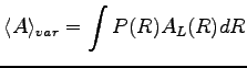
The VMC is a stochastic method that allows to evaluate expectation values of physical operators on a given wave-function (see Ref. (26)). It is based on a statistical calculation of
the integrals that involve the mean values of these operators.
 |
(1.1) |
where
 are the electron coordinates.
Monte Carlo integration is necessary because the wave-function contains explicit particle correlations and this leads to non-factoring multi-dimension integrals.
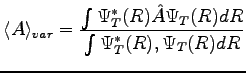
Notice that in the case of the Hamiltonian operator, according to the variational principle, the expectation value will be greater than or equal to the exact ground state energy.
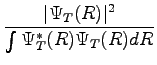
We can write the integral 1.1 as:
are the electron coordinates.
Monte Carlo integration is necessary because the wave-function contains explicit particle correlations and this leads to non-factoring multi-dimension integrals.
Notice that in the case of the Hamiltonian operator, according to the variational principle, the expectation value will be greater than or equal to the exact ground state energy.
We can write the integral 1.1 as:
where  in a probability density, and
  is the diagonal element associated to the operator
  .
.
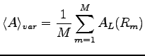
We can sample the probability distribution
using the Metropolis scheme (27) and then evaluate
on the obtained configurations. Then using the central limit theorem the integral can be estimate as:
The sampling process continues until the desired statistical error on the expectation value of the operator
is reached.
The VMC algorithm is implemented so that only a single electron is moved at each time.
In this way only one column or one row of the Pair Determinant is changed at each step.
The new determinant can be computed in
 operations, given the inverse of the old pair determinant. This inverse is computed once at the beginning of the simulation and then updated whenever a trial move is accepted. If the trial move is accepted, the inverse matrix is updated in
 operations. This trick makes the VMC sampling very efficient. Notice that the direct computation of a determinant takes
 operations.
Subsections
Next: Forces with finite variance
Up: Quantum Monte Carlo and
Previous: Quantum Monte Carlo and
Contents
Claudio Attaccalite
2005-11-07