Practical implementation of the finite temperature dynamics

In the same spirit of the Car-Parrinello dynamics, at each ionic move, eq. 5.22, the parameters are optimized using eq. 2.31. This has allowed us to relax the wave-function to the energy minimum during the ionic dynamics . We call this technique Generalized Langevin Dynamics using Quantum Monte Carlo noisy forces(GLQ).
In order to simulate finite temperature systems using the GQL dynamics some control parameters has to be fixed for an efficient scheme. Let us imagine that we want to simulate a system at given temperature $T$ and density $r_S$ . First of all we have to choose the friction tensor. Two choices are possible: the first one is to work with the friction as small as possible, compatibly with the QMC noise, in order not to affect dynamic properties; the second choice is to choose the friction in such a way to achieve the maximum convergence speed. In this thesis we did not investigate dynamical properties and so we opted for the second choice. Second, we have to determine the two parameters $r$ and $\Delta$ see eq. 2.33 and 5.22. We have chosen $r$ as big as possible to have a stable optimization. Instead $\Delta$ has been chosen enough small to allow the Hessian optimization to follow the ionic dynamics. This can be easily checked controlling if the forces 2.11 are zero within a given accuracy. For example for a system of $16$ hydrogen atoms we have used a time step $\Delta$ of the order of $0.3 fs$ for a temperature around $100K$ . For higher temperature in order to maintain the same precision between ionic dynamics and optimization of parameters the time step $\Delta$ is roughly rescaled as $\sim{1/\sqrt{T}}$ in such a way to maintain the same mean ionic step $\langle \left\vert \Delta R \right\vert \rangle \sim \sqrt{\langle v^2 \rangle} \Delta$ . Moreover to have a stable minimization not all parameters have to be changed at each ionic step but only the most relevant, see the forthcoming section 5.4.3.
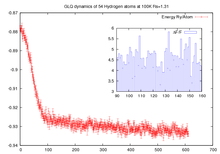
Thanks to GLQ technique we were able to simulate reasonably large systems, by using highly correlated wave-functions with many parameters (see figure 5.1) and with essentially a single processor machine.

Figure 5.1: Ionic dynamics of 54 hydrogen atoms using GLQ, with a time step $0.4 fs$ , starting from a BCC lattice. The trial wave-function contains 2920 variational parameters and we have optimized 300 of them at each step. In the inset the maximum deviation $F_i/\Delta F_i$ of the forces acting on the variational parameters is shown.