


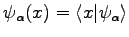
Next: Results on Molecules
Up: Optimization Methods
Previous: Structural optimization
Contents
Hessian Optimization
The SR method generally performs very well,
whenever there is only one energy scale in the
variational wave function.
However if there are several energy scales in the problem,
some of the variational parameters, e.g. the ones defining the
low energy valence orbitals, converge very slowly with respect to the
others, and the number
of iterations required for the equilibration becomes exceedingly large. Moreover
the time step  necessary for a stable
convergence depends
on the high energy orbitals, whose dynamics cannot be accelerated beyond a
certain threshold.
Futhermore the SR method is based on a first order dynamics, and as will be illustrated in the following (see section 5.4.2), it is not adapted to perform parameters optimization during a ion Langevin Dynamics.
In this thesis to overcome these difficulties we have used a very efficient optimization method the Stochastic Reconfiguration with Hessian acceleration (SRH) (50).
necessary for a stable
convergence depends
on the high energy orbitals, whose dynamics cannot be accelerated beyond a
certain threshold.
Futhermore the SR method is based on a first order dynamics, and as will be illustrated in the following (see section 5.4.2), it is not adapted to perform parameters optimization during a ion Langevin Dynamics.
In this thesis to overcome these difficulties we have used a very efficient optimization method the Stochastic Reconfiguration with Hessian acceleration (SRH) (50).
The central point of the SRH is to use not only directions given by the generalized forces 2.11, to lower the energy expectation value, but also the information coming from the Hessian matrix to accelerate the convergence. The idea to use the Hessian matrix is not new, already Lin, Zhang and Rappe (45) proposed to use analytic derivatives to optimize the energy, but their implementation was inefficient and unstable.
Now we will review the SRH method and we will explain the reason of its efficiency.
Given an Hamiltonian  and a trial-function
 depending on a set of parameters
 , we want to optimize the energy expectation value of the energy on this wave-function:
 |
(2.24) |
respect to the parameters set.
To simplify the notation henceforth the symbol  indicates the quantum expectation value over
 , so that
 . In order the optimize the energy and to find the new parameters
 , we expand the trial-function up to second order in
  :
:
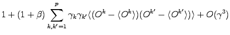
![$\displaystyle \vert\psi_{\alpha+\gamma} \rangle = \left \{ 1 + \left [ \sum_k^p...
...)(O^{k'} -\langle O^{k'} \rangle) \right] \right \} \vert \psi_{\alpha} \rangle$](img287.png) |
(2.25) |
with  , where
  is the operator with associated diagonal elements (15):
 |
(2.26) |
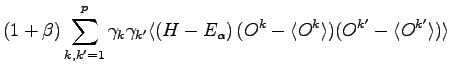
Here the constant  will be used in order to highlight the various terms in the energy expansions. Using the fact that:
we can expand up second order the energy given by the new wave-function
 and obtain:
We can define:
and so the expansion of the energy reads:
![$\displaystyle \Delta E = - \sum_k \gamma_k f_k + \frac{1}{2} \sum_{k,k'} \left ( 1+ \beta \right ) \left [ S_h + ( 1 + \beta ) G \right ]^{k,k'}$](img308.png) |
(2.30) |
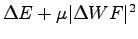
The wave-function parameters can then iteratively changed to stay at the minimum of the above quadratic form whenever it is positive defined, and in such case the minimum energy is obtained for:
 |
(2.31) |
where
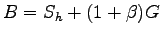 |
(2.32) |
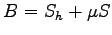
It can happen that the quadratic form is not positive definite and so the energy expansion 2.30 is not bounded from below, this can due to different reasons: non quadratic corrections; statistical fluctuations of the Hessian matrix expectation value; or because we are far from the minimum. In this cases the correction due to the equation 2.31 may lead to an higher energy than  . To overcame this problem the matrix
  is changed in such way to be always positive definite
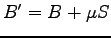 , where
  is the Stochastic Reconfiguration matrix 2.9. The use of the
matrix guarantees that we are moving in the direction of a well defined minimum when the change of the wave-function is small, moreover in the limit of large
is the Stochastic Reconfiguration matrix 2.9. The use of the
matrix guarantees that we are moving in the direction of a well defined minimum when the change of the wave-function is small, moreover in the limit of large  we recover the Stochastic Reconfiguration optimization method.
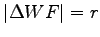
To be sure that the change of the wave-function is small we use a control parameter to impose a constraint to the variation of the wave-function
we recover the Stochastic Reconfiguration optimization method.
To be sure that the change of the wave-function is small we use a control parameter to impose a constraint to the variation of the wave-function  by means of the inequalities
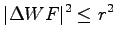 |
(2.33) |
where, using 2.9 and 2.25,
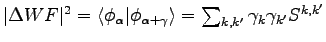 .
This constraint always allows to work with a positive definitive matrix
.
This constraint always allows to work with a positive definitive matrix  , and for small
  the energy is certainly lower than
. We want to emphasize that the condition
the energy is certainly lower than
. We want to emphasize that the condition
 is non zero both when 2.32 is not positive defined and when
 corresponding to eq. 2.31 exceeds
. This is equivalent to impose a Lagrange multiplier to the energy minimization, namely
corresponding to eq. 2.31 exceeds
. This is equivalent to impose a Lagrange multiplier to the energy minimization, namely
 , with the condition
 .
.
There is another important ingredients for an efficient implementation of the Hessian technique to QMC. In fact, as pointed out in Ref.(58,50) is extremely important to evaluate the quantities appearing in the Hessian 2.32 in the form of correlation function
 . This because the fluctuation of operators in this form are usually smaller than the one of
  especially if
  and
are correlated. Therefore using the fact that the expectation value of the derivative of a local value
and
are correlated. Therefore using the fact that the expectation value of the derivative of a local value
 of an Hermitian operator
  respect to any real parameter
  in a real wave function
  is always zero (see for instance (45)), we can rearrange the Hessian terms in more symmetric way in form of correlation function:
Because the  matrix 2.28 is zero for the exact ground state and therefore is expected to be very small for a good variational wave-function, it is possible, following the suggestion of Ref. (50), to chose
 , so that
 . As shown by Ref. (50) this choice can even lead to faster convergence than the full Hessian matrix.
The matrix
is the only part that is not in the form of a correlation function, for this reason is important that
does not depend on it, in such way to reduce the fluctuation of the Hessian matrix, and this can naively explain the suggestion of Ref. (50) to chose
.
As for the SR method the parameters are iteratively updated using the equation:
![$\displaystyle \vec{\gamma} = \left [ S_h + \mu S \right ]^{-1} \vec{f}$](img336.png) |
(2.34) |
where the forces  and the matrix
are evaluated using VMC.
and the matrix
are evaluated using VMC.
Next: Results on Molecules
Up: Optimization Methods
Previous: Structural optimization
Contents
Claudio Attaccalite
2005-11-07
![$\displaystyle \frac{1}{2} \langle \left [ O^{k} -\langle O^{k} \rangle , \left [ H -E_\alpha , O^{k} -\langle O^{k} \rangle \right ]\right] \rangle$](img301.png)