NEW TUTORIAL FOR YAMBO 4.4:
Real-time Bethe Salpeter Equation
This tutorial will show how to perform a simple real-time BSE calculation with Yambo 4.4 on hBN monolayer. DFT inputs are available here: QE_inputs or ABINIT_inputs. Follow the first 6 steps of the linear-response tutorial. Then generate the input file to calculate the collisions (see appendix of Phys. Rev. B 84, 245110): yambo_nl -b -e -v h+sex. The flag -b will tell the code to calculate the dielectric constant that is required for the screened interaction.
em1s                           # [R Xs] Static Inverse Dielectric Matrix
collisions                     # [R] Eval the extended Collisions
dipoles                        # [R   ] Compute the dipoles
DIP_Threads=0                  # [OPENMP/X] Number of threads for dipoles
X_Threads=0                    # [OPENMP/X] Number of threads for response functions
RT_Threads=0                   # [OPENMP/RT] Number of threads for real-time
Chimod= "HARTREE"              # [X] IP/Hartree/ALDA/LRC/PF/BSfxc
% BndsRnXs
   1 |  40 |                   # [Xs] Polarization function bands
%
NGsBlkXs= 1000 mHa      # [Xs] Response block size
% DmRngeXs
  0.10000 |  0.10000 | eV      # [Xs] Damping range
%
% LongDrXs
 1.000000 | 0.000000 | 0.000000 |        # [Xs] [cc] Electric Field
%
% COLLBands
   4 |  5 |                   # [COLL] Bands for the collisions
%
HXC_Potential= "HARTREE+SEX"           # [SC] SC HXC Potential
HARRLvcs= 1000 mHa      # [HA] Hartree     RL components
EXXRLvcs= 1000 mHa      # [XX] Exchange    RL components
CORRLvcs= 1000 mHa      # [GW] Correlation RL components
With this input we calculate the HARTREE and SEX collisions integrals. Notice that the HARTREE term in principle can be calculate on the fly, but in this way it is more efficiend expecially for the non-linear response. Here one has to converge the cutoff for the Hartree and the Screened Exchange, usually 5000 mHa it is a good value, in this example I put 1000 mHa to speed up calculations. The collisions bands COLLBands have to be the same number of bands you want to use in the linear/nonlinear response. Run this calculation, it will take 5 minutes on a serial PC.
Then you generate the input for the linear response yambo_nl -u -V qp :
nloptics                       # [R NL] Non-linear optics
DIP_Threads=0                  # [OPENMP/X] Number of threads for dipoles
NL_Threads=0                   # [OPENMP/NL] Number of threads for nl-optics
% NLBands
  4 |  5 |                     # [NL] Bands
%
NLverbosity= "low"             # [NL] Verbosity level (low | high)
NLstep=   0.0100       fs      # [NL] Real Time step length
NLtime= 55.00000       fs      # [NL] Simulation Time
NLintegrator= "CRANKNIC"         # [NL] Integrator ("EULEREXP/RK2/RK4/RK2EXP/HEUN/INVINT/CRANKNIC")
NLCorrelation= "SEX"           # [NL] Correlation ("IPA/HARTREE/TDDFT/LRC/LRW/JGM/SEX")
NLLrcAlpha= 0.000000           # [NL] Long Range Correction
% NLEnRange
 0.200000 | 8.000000 | eV      # [NL] Energy range
%
NLEnSteps= 1                   # [NL] Energy steps
NLDamping=  0.10000    eV      # [NL] Damping
#UseDipoles                    # [NL] Use Covariant Dipoles (just for test purpose)
#FrSndOrd                      # [NL] Force second order in Covariant Dipoles
#EvalCurrent                   # [NL] Evaluate the current
HARRLvcs= 1017         RL      # [HA] Hartree     RL components
EXXRLvcs= 1074         mHa     # [XX] Exchange    RL components
% ExtF_Dir
 0.000000 | 1.000000 | 0.000000 |        # [NL ExtF] Versor
%
ExtF_Int= 1000.        kWLm2   # [NL ExtF] Intensity
ExtF_Width= 0.000000   fs      # [NL ExtF] Field Width
ExtF_kind= "DELTA"             # [NL ExtF] Kind(SIN|SOFTSIN|RES|ANTIRES|GAUSS|DELTA|QSSIN)
ExtF_Tstart=   0.0100  fs      # [NL ExtF] Initial Time
% GfnQP_E
 3.000000 | 1.000000 | 1.000000 |        # [EXTQP G] E parameters  (c/v) eV|adim|adim
%
Notice that we introduced a scissor operator (a rigid shif of the conduction bands) of 3.0 eV. In principle it is possible to perform a G0W0 calculation with Yambo and use the Quasi-particle band structure instead of the rigid shift.
Run this calculation and then anlize the result in the same way of linear reponse tutorial, you will get a nice excitons in hBN, as the one plotted below in the old tutorial. You can repeat the same kind of calculations for the non-linear response.
OLD LUMEN TUTORIAL:
Real-time Bethe Salpeter Equation
This tutorial will show how to perform a simple real-time BSE calculation with lumen on hBN monolayer. DFT inputs are available here: QE_inputs or ABINIT_inputs.
Follow the same steps of the linear-response tutorial, but when you generate the lumen input file use: lumen -u -V qp -b. The flag -b will tell the code to calculate the dielectric constant that is required for the screened interaction. Then you set:
nlinear                      # [R NL] Non-linear optics
em1s                         # [R Xs] Static Inverse Dielectric Matrix
Chimod= "hartree"            # [X] IP/Hartree/ALDA/LRC/BSfxc
% BndsRnXs
   1 |  20 |                 # [Xs] Polarization function bands
%
NGsBlkXs= 5           RL    # [Xs] Response block size
% DmRngeXs
  0.10000 |  0.10000 | eV    # [Xs] Damping range
%
% LongDrXs
 0.000    |0.1000E-4 | 0.000    |        # [Xs] [cc] Electric Field
%
% NLBands
  4 |  5 |                   # [NL] Bands
%
NLstep=   0.0100       fs    # [NL] Real Time step length
NLtime= 55.00000       fs    # [NL] Simulation Time
NLverbosity= "high"           # [NL] Verbosity level (low | high)
NLintegrator= "CRANKNIC"     # [NL] Integrator ("EULEREXP/RK4/RK2EXP/HEUN/INVINT/CRANKNIC")
NLCorrelation= "SEX"        # [NL] Correlation ("IPA/HARTREE/TDDFT/LRC/JGM/SEX/HF")
NLLrcAlpha= 0.000000         # [NL] Long Range Correction
% NLEnRange
 0.200000 | 8.000000 | eV    # [NL] Energy range
%
NLEnSteps= 1                 # [NL] Energy steps
NLDamping=  0.10000    eV    # [NL] Damping
NLGvecs= 107           RL    # [NL] Number of G vectors in NL dynamics for Hartree/TDDFT
% ExtF_Dir
 0.000000 | 1.000000 | 0.000000 |        # [NL ExtF] Versor
%
ExtF_kind= "DELTA"           # [NL ExtF] Kind(SIN|SOFTSIN|RES|ANTIRES|GAUSS|DELTA|QSSIN)
GfnQPdb= "none"              # [EXTQP G] Database
GfnQP_N= 1                   # [EXTQP G] Interpolation neighbours
% GfnQP_E
 3.000000 | 1.000000 | 1.000000 |        # [EXTQP G] E parameters  (c/v) eV|adim|adim
%
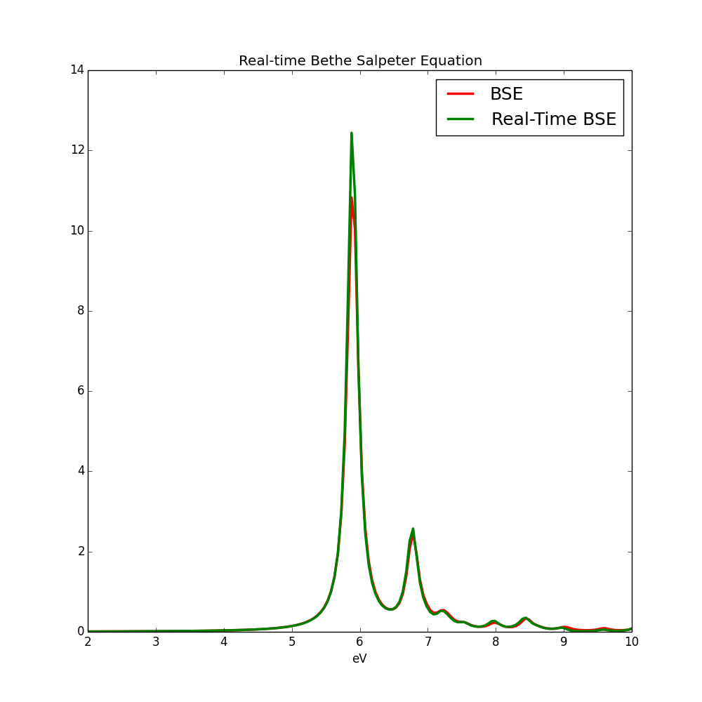
Notice that in the calculation we decreased the number of g-vectors in the Hartree term, NLGvecs to speed up calculation,in case of BN this does not change the result because local field effects are very small in h-BN along the plane.Now you can analyze the response with ypp as it was done the linear response tutorial and compare with the standard Bethe-Salpeter (input here):