Correlation and Second Harmonic Generation
In this tutorial we will show how to include correlation effects in the Second Harmonic Generation. We start from the tutorial on SHG in AlAs, using the same DFT inputs and parameters.
Notice that the tutorials on TD-Hartree, TD-DFT and TD-DPFT require more computational time, if calculations are too slow you can run in parallel or decrease the number of frequencies in your SHG.
1) Quasi-particle corrections
Quasi-particle correction can be easily introduced in the real-time dynamics by means of a non-local operator that modifies the Kohn-Sham eigenvalues: $$ \Delta \hat H = \sum_{n,\bf k} \Delta_{n,\bf k} |v^0_{n,\bf k}\rangle\langle v^0_{n,\bf k}|. $$ The command to turn on quasi-particle corrections is: "yambo_nl -u -V qp" :
All the parameters of this input are the same of the previous tutorial with the only difference that we introduced a scissor operator of 0.9 eV. Notice that it is possible to import also the quasi-particle corrections calculated within the G0W0 approximation by using the flag
GfnQPdb="E < SAVE/ndb.QP" (see Yambo tutorial on GW for more information). Now you can run lumen and then analyze the results as explained in the previous tutorial. The effect of then scissor-operator is shown in the following figure:
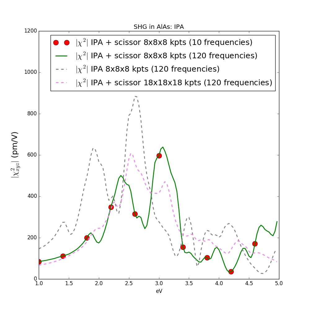
The figure compares results with scissor operator "IPA + scissor" (red dots) with the one obtained in the previous tutorial "IPA". The full converged result is obtained with a 18x18x18 k-point grid and bands between 2 and 10 (violet dashed line). The script and the data to generate this plot can be downloaded here.
2) Time-dependent Hartree (RPA wih local field effects)
In order to include local field effects in the SHG we use the Time-dependent Hartree approximation, see the theory page for more details. The input is generated with the usual command "lumen -u -V RL" where we turned on the Reciprocal Lattice vectors verbosity in order to specify the number of plane wave to use in the calculations. To run a TD-Hartree calculation you just specify NLCorrelation="HARTREE" and then we reduce the number of plane waves to 307, that is enough to have a converged result in this system.
In this run we increase the damping to 0.25 eV in such a way to speed up calculations. The result of this calculation is shown in the figure below: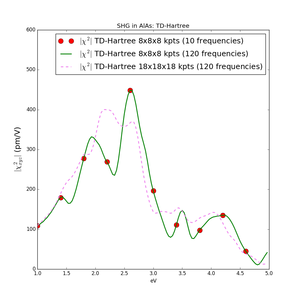
3) Time-dependent Density Functional Theory (TD-DFT)
TD-DFT calculations are similar to the TD-Hartree ones. Just change NLCorrelation="TDDFT" and the exchange correlation functional used in the ground state calculations will be included in the real-time dynamics. Notice that only LDA or GGA functionals are supported by Yambo/Lumen. These functionals usually provide an insignificant improvement respect to the TD-Hartree because they miss the long-range part that will be included in the next tutorial by means of TD-DPFT theory. You can perform TD-DFT calculations as exercise and compare with the other approximations.
The converged result on a 18x18x18 k-points grid is reported below: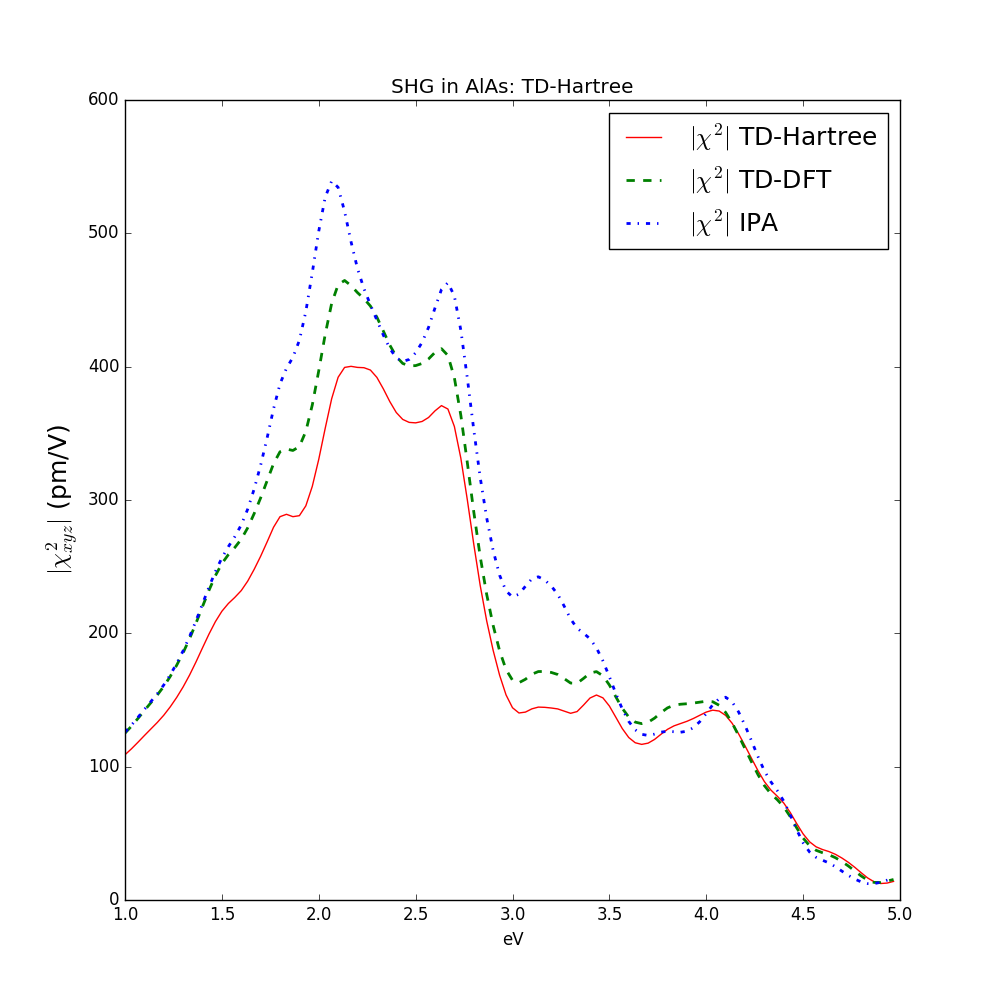
4) Time-dependent Density-Polarization Functional Theory (TD-DPFT)
In this last tutorial on SHG we will include both quasi-particle effects by means of a scissor operator and long-range correction to the response function by means of Time-dependent Density-Polarization Functional Theory. The Lumen input can be generated as usual with the command lumen -u -V qp:
The \( \alpha \) parameter for AlAs has been suggested by Botti and coworkers in PRB 69, 155112. The results is: 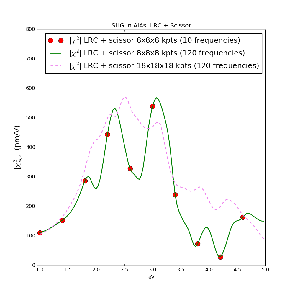
Plot data are available here.
Notice that different models for the \( \alpha \) parameter have been proposed in the literature, see PRB 94 035149 (2016) for a discussion.
Finally in Yambo we implemented also the Jelium-with gap model NLCorrelation="JGM" that provides an automatic estimation of the \( \alpha \) parameters for each material, see M. Grüning, D. Sangalli, C. Attaccalite, Phys. Rev. B 94, 035149 (2016) for a discussion on this approximation.
Notice that the tutorials on TD-Hartree, TD-DFT and TD-DPFT require more computational time, if calculations are too slow you can run in parallel or decrease the number of frequencies in your SHG.
1) Quasi-particle corrections
Quasi-particle correction can be easily introduced in the real-time dynamics by means of a non-local operator that modifies the Kohn-Sham eigenvalues: $$ \Delta \hat H = \sum_{n,\bf k} \Delta_{n,\bf k} |v^0_{n,\bf k}\rangle\langle v^0_{n,\bf k}|. $$ The command to turn on quasi-particle corrections is: "yambo_nl -u -V qp" :
nlinear                      # [R NL] Non-linear optics
% NLBands
  3 |  6 |                   # [NL] Bands
%
NLintegrator="INVINT"       # [NL] Integrator ("EULEREXP/RK4/RK2EXP/HEUN/INVINT/CRANKNIC")
NLCorrelation= "IPA"         # [NL] Correlation ("IPA/HARTREE/TDDFT/LRC/JGM/SEX/HF")
NLLrcAlpha= 0.000000         # [NL] Long Range Correction
% NLEnRange
 1.000000 | 5.000000 | eV    # [NL] Energy range
%
NLEnSteps= 10                # [NL] Energy steps
NLDamping= 0.150000    eV    # [NL] Damping
% ExtF_Dir
 1.000000 | 1.000000 | 0.000000 |        # [NL ExtF] Versor
%
ExtF_kind= "SOFTSIN"         # [NL ExtF] Kind(SIN|SOFTSIN|RES|ANTIRES|GAUSS|DELTA|QSSIN)
GfnQPdb= "none"              # [EXTQP G] Database
GfnQP_N= 1                   # [EXTQP G] Interpolation neighbours
% GfnQP_E
 0.900000 | 1.000000 | 1.000000 |        # [EXTQP G] E parameters  (c/v) eV|adim|adim
%
GfnQP_Z= ( 1.000000 , 0.000000 )       # [EXTQP G] Z factor  (c/v)
GfnQP_Wv_E= 0.000000   eV    # [EXTQP G] W Energy reference  (valence)
% GfnQP_Wv
 0.00     | 0.00     | 0.00     |        # [EXTQP G] W parameters  (valence) eV| eV|eV^-1
%
GfnQP_Wc_E= 0.000000   eV    # [EXTQP G] W Energy reference  (conduction)
% GfnQP_Wc
 0.00     | 0.00     | 0.00     |        # [EXTQP G] W parameters  (conduction) eV| eV|eV^-1
%
All the parameters of this input are the same of the previous tutorial with the only difference that we introduced a scissor operator of 0.9 eV. Notice that it is possible to import also the quasi-particle corrections calculated within the G0W0 approximation by using the flag
GfnQPdb="E < SAVE/ndb.QP" (see Yambo tutorial on GW for more information). Now you can run lumen and then analyze the results as explained in the previous tutorial. The effect of then scissor-operator is shown in the following figure:
2) Time-dependent Hartree (RPA wih local field effects)
In order to include local field effects in the SHG we use the Time-dependent Hartree approximation, see the theory page for more details. The input is generated with the usual command "lumen -u -V RL" where we turned on the Reciprocal Lattice vectors verbosity in order to specify the number of plane wave to use in the calculations. To run a TD-Hartree calculation you just specify NLCorrelation="HARTREE" and then we reduce the number of plane waves to 307, that is enough to have a converged result in this system.
nlinear                      # [R NL] Non-linear optics
% NLBands
  3 |  6 |                   # [NL] Bands
%
NLintegrator="INVINT"       # [NL] Integrator ("EULEREXP/RK4/RK2EXP/HEUN/INVINT/CRANKNIC")
NLCorrelation= "HARTREE"         # [NL] Correlation ("IPA/HARTREE/TDDFT/LRC/JGM/SEX/HF")
NLLrcAlpha= 0.000000         # [NL] Long Range Correction
% NLEnRange
 1.000000 | 5.000000 | eV    # [NL] Energy range
%
NLEnSteps= 10                # [NL] Energy steps
HARRLvcs=  105         RL      # [HA] Hartree     RL components
EXXRLvcs=  105         RL      # [XX] Exchange    RL components
NLDamping= 0.250000    eV    # [NL] Damping
% ExtF_Dir
 1.000000 | 1.000000 | 0.000000 |        # [NL ExtF] Versor
%
ExtF_kind= "SOFTSIN"         # [NL ExtF] Kind(SIN|SOFTSIN|RES|ANTIRES|GAUSS|DELTA|QSSIN)
In this run we increase the damping to 0.25 eV in such a way to speed up calculations. The result of this calculation is shown in the figure below:
3) Time-dependent Density Functional Theory (TD-DFT)
TD-DFT calculations are similar to the TD-Hartree ones. Just change NLCorrelation="TDDFT" and the exchange correlation functional used in the ground state calculations will be included in the real-time dynamics. Notice that only LDA or GGA functionals are supported by Yambo/Lumen. These functionals usually provide an insignificant improvement respect to the TD-Hartree because they miss the long-range part that will be included in the next tutorial by means of TD-DPFT theory. You can perform TD-DFT calculations as exercise and compare with the other approximations.
The converged result on a 18x18x18 k-points grid is reported below:
4) Time-dependent Density-Polarization Functional Theory (TD-DPFT)
In this last tutorial on SHG we will include both quasi-particle effects by means of a scissor operator and long-range correction to the response function by means of Time-dependent Density-Polarization Functional Theory. The Lumen input can be generated as usual with the command lumen -u -V qp:
nlinear                      # [R NL] Non-linear optics
% NLBands
  3 | 6 |                   # [NL] Bands
%
NLintegrator="INVINT"       # [NL] Integrator ("EULEREXP/RK4/RK2EXP/HEUN/INVINT/CRANKNIC")
NLCorrelation= "LRC"     # [NL] Correlation ("IPA/HARTREE/TDDFT/LRC/JGM")
NLLrcAlpha= 0.350000         # [NL] Long Range Correction
% NLEnRange
 0.200000 | 8.000000 | eV    # [NL] Energy range
%
NLEnSteps= 10               # [NL] Energy steps
HARRLvcs=  105         RL      # [HA] Hartree     RL components
EXXRLvcs=  105         RL      # [XX] Exchange    RL components
NLDamping= 0.150000    eV    # [NL] Damping
% ExtF_Dir
 1.000000 | 1.000000 | 0.000000 |        # [NL ExtF] Versor
%
ExtF_kind= "SOFTSIN"         # [NL ExtF] Kind(SIN|SOFTSIN|RES|ANTIRES|GAUSS|DELTA|QSSIN)
GfnQPdb= "none"              # [EXTQP G] Database
GfnQP_N= 1                   # [EXTQP G] Interpolation neighbours
% GfnQP_E
 0.900000 | 1.000000 | 1.000000 |        # [EXTQP G] E parameters  (c/v) eV|adim|adim
%
The \( \alpha \) parameter for AlAs has been suggested by Botti and coworkers in PRB 69, 155112. The results is:
Notice that different models for the \( \alpha \) parameter have been proposed in the literature, see PRB 94 035149 (2016) for a discussion.
Finally in Yambo we implemented also the Jelium-with gap model NLCorrelation="JGM" that provides an automatic estimation of the \( \alpha \) parameters for each material, see M. Grüning, D. Sangalli, C. Attaccalite, Phys. Rev. B 94, 035149 (2016) for a discussion on this approximation.