Stabilization of the SR technique

Whenever the number of variational parameters increases, it often happens that the stochastic $N\times N$ matrix

$$s_{k,k^\prime} ={ \langle \Psi \vert O_k O_{k^\prime} \vert \Psi\... ...si \vert O_{k^\prime} \vert \Psi\rangle \over \langle \Psi \vert \Psi \rangle }$$ (2.16)

becomes singular, i.e. the condition number, defined as the ratio $\sigma=\lambda_N/\lambda_1$ between its maximum $\lambda_N$ and minimum eigenvalue $\lambda_1$ , is too large. In that case the inversion of this matrix generates clear numerical instabilities which are difficult to control especially within a statistical method.

The first successful proposal to control this instability was to remove from the inversion problem (49), required for the minimization, those directions in the variational parameter space corresponding to exceedingly small eigenvalues $\lambda_i$ . In this thesis we describe a method the is much better. As a first step, we show that the reason of the large condition number $\sigma$ is due to the existence of ''redundant'' variational parameters that do not make changes to the wave function within a prescribed tolerance $\epsilon$ .

Indeed in practical calculations, we are interested in the minimization of the wave function within a reasonable accuracy. The tolerance $\epsilon$ may represent therefore the distance between the exact normalized variational wave function which minimizes the energy expectation value and the approximate acceptable one, for which we no longer iterate the minimization scheme. For instance $\epsilon=1/1000$ is by far acceptable for chemical and physical interest.

A stable algorithm is then obtained by simply removing the parameters that do not change the wave function by less than $\epsilon$ from the minimization. An efficient scheme to remove the ''redundant parameters'' is also given.

Let us consider the $N$ normalized states orthogonal to $\Psi$ , but not mutually orthogonal:

$$\vert e_i\rangle = { (O_k - \langle O_k \rangle ) \vert \Psi \rangle \over \sqrt { \langle \Psi \vert (O_k - \langle O_k \rangle )^2 \vert\Psi } }.$$ (2.17)

These normalized vectors define $N$ directions in the $N-$ dimensional variational parameter manifold, which are independent as long as the determinant $S$ of the corresponding $N\times N$ overlap matrix

$$s_{k,k^\prime} = \langle e_k \vert e_{k^\prime} \rangle$$ (2.18)

$$\langle e_k \vert e_k \rangle = 1$$ (2.19)

is non zero. The number $S$ is clearly positive and it assumes its maximum value $1$ whenever all the directions $e_i$ are mutually orthogonal. On the other hand, let us suppose that there exists an eigenvalue $\bar \lambda$ of $s$ smaller than the square of the desired tolerance $\epsilon^2$ , then the corresponding eigenvector $\vert v>=\sum_i a_i \vert e_i\rangle$ is such that:

$$\langle v \vert v \rangle = \sum_{i,j} a_i a_j \bar s_{i,j} = \bar \lambda$$ (2.20)

where the latter equation holds due to the normalization condition $\sum_i a_i^2 =1$ . We arrive therefore to the conclusion that it is possible to define a vector $v$ with almost vanishing norm $\vert v\vert =\sqrt{\lambda} \le \epsilon$ as a linear combination of $e_i$ , with at least some non zero coefficient. This implies that the $N$ directions $e_k$ are linearly dependent within a tolerance $\epsilon$ and one can safely remove at least one parameter from the calculation.

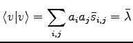
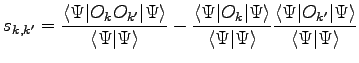
In general whenever there are $p$ vectors $v_i$ that are below the tolerance $\epsilon$ the optimal choice to stabilize the minimization procedure is to remove $p$ rows and $p$ columns from the matrix (2.18), in such a way that the corresponding determinant of the $(N-p) \times (N-p)$ overlap matrix is maximum.

From practical purposes it is enough to consider an iterative scheme to find a large minor, but not necessarily the maximum one. This method is based on the inverse of $\bar s$ . At each step we remove the $i-th$ row and column from $\bar s$ for which $\bar s^{-1}_{i,i}$ is maximum. We stop to remove rows and columns after $p$ inversions. In this approach we exploit the fact that, by a consequence of the Laplace theorem on determinants, $\bar s^{-1}_{k,k}$ is the ratio between the described minor without the $k-th$ row and column and the determinant of the full $\bar s$ matrix. Since within a stochastic method it is certainly not possible to work with a machine precision tolerance, setting $\epsilon=0.001$ guarantees a stable algorithm, without affecting the accuracy of the calculation. The advantage of this scheme, compared with the previous one(18), is that the less relevant parameters can be easily identified after few iterations and do not change further in the process of minimization.